Keystroke Dynamics - Lab vs Field Data

On this webpage, we share the data, scripts, and results of our evaluation so that other researchers can use the data, reproduce our results, and extend them; or, use the data for investigations of related topics, such as intrusion, masquerader or insider detection. We hope these resources will be useful to the research community.

Common questions:

• Q1-1: What is keystroke dynamics (or keystroke biometrics)?
Keystroke dynamics is the study of whether people can be distinguished by their typing rhythms, much like handwriting is used to identify the author of a written text. Possible applications include acting as an electronic fingerprint, or in an access-control mechanism. A digital fingerprint would tie a person to a computer-based crime in the same manner that a physical fingerprint ties a person to the scene of a physical crime. Access control could incorporate keystroke dynamics both by requiring a legitimate user to type a password with the correct rhythm, and by continually authenticating that user while they type on the keyboard.
• Q1-2: What is your paper about? What is this webpage for?
In the field of keystroke dynamics, there are many different methods of collecting timing data from subjects. A data collection program can run in the browser, separate copies of the program can run on the personal computer of each subject, or a single program can run on one computer in a laboratory setting. In our paper, we show that collecting data outside of the laboratory setting can result in low-quality data.

Our intent with this webpage is to share our resources—the typing data, evaluation scripts, and the table of results—with the research community, and to answer questions that they (or you) might have.
• Q1-3: Where can I find a copy of the paper?
The paper is included in the Proceedings of CONFERENCE NAME (CONF-DATE) Conference, published by PUBLISHER [1].
• Q1-4: How would I cite this webpage in a publication?
This webpage is a supplement to our original paper in CONF-DATE, and the paper refers readers to this website. Consequently, we ask authors who find this web resource useful provide a citation to the original paper [1]. See the citation in Section 5, References, at the end of this web page.

This section presents two datasets: one collected in our lab and one collected in the field. The data for both consist of keystroke-timing information from 100 subjects (typists), each typing a password (.tie5Roanl) 400 times.

Lab:
• lab_dataset.txt (Fixed-width format) ................... MD5 hash = ??
• lab_dataset.csv (Comma-separated-value format) MD5 hash = ??
• lab_dataset.xls (Excel format) ............................. MD5 hash = ??

Field:
• field_dataset.txt (Fixed-width format) ................... MD5 hash = ??
• field_dataset.csv (Comma-separated-value format) MD5 hash = ??
• field_dataset.xls (Excel format) ............................. MD5 hash = ??

Common questions:

• Q2-1: How were the data collected?

For complete details of our data collection methodology, we refer readers to our original paper [1]. A brief summary of our methodology follows.

Lab:

We built a keystroke data-collection apparatus consisting of: (1) a laptop running Windows XP; (2) a Windows software application for presenting stimuli to the subjects, and for recording their keystrokes; and (3) an external reference timer for timestamping those keystrokes. The software presents the subject with the password to be typed. As the subject types the password, it is checked for correctness. If the subject makes a typographical error, the application prompts the subject to retype the password. In this manner, we record timestamps for 50 correctly typed passwords in each session.

Whenever the subject presses or releases a key, the software application records the event (i.e., keydown or keyup), the name of the key involved, and a timestamp for the moment at which the keystroke event occurred. An external reference clock was used to generate highly accurate timestamps. The reference clock was demonstrated to be accurate to within ±200 microseconds (by using a function generator to simulate key presses at fixed intervals).

We recruited 100 subjects (typists) from within a university community. All subjects typed the same password, and each subject typed the password 400 times over 8 sessions (50 repetitions per session). They waited at least one day between sessions, to capture some of the day-to-day variation of each subject's typing. The password (.tie5Roanl) was chosen to be representative of a strong 10-character password.

The raw records of all the subjects' keystrokes and timestamps were analyzed to create a password-timing table. The password-timing table encodes the timing features for each of the 400 passwords that each subject typed.

Field:

The same Windows application used to collect data for our lab dataset was adapted to run on the personal computer of each subject in our field dataset. Keystrokes were timestamped using two onboard timers available to Windows programs: the Query Performance Counter (QPC) for high-resolution timestamps and the Tick Timer for standard, low-resolution timestamps. Only timing data from the QPC is presented in the field dataset; the Tick Timer timestamps were used for sanity-checking our results.

We recruited 100 subjects from various university communities. All 100 subjects are distinct from the subjects in the lab dataset—there are no subjects who contributed to both datasets. As in the lab dataset, all subjects typed the same password (.tie5Roanl), and each subject typed the password 400 times over 8 sessions (50 repetitions per session).

The password-timing table for the field data was generated from the raw data in the same manner as the password-timing table for the lab data. Likewise, the field data password-timing table encodes the timing features for each of the 400 passwords that each subject typed.

• Q2-2: How do I read the data into R / Matlab / Weka / Excel / ...?
  The data are provided in three different formats to make it easier for researchers visiting this page to view and manipulate the data. In all its forms, the data are organized into a table, but different applications are better suited to different formats.
  
  (R): In the fixed-width format, the columns of the table are separated by one or more spaces so that the information in each column is aligned vertically. This format is easy to read in a standard web browser or document editor with a fixed width font. It can also be read by the standard data-input mechanisms of the statistical-programming environment R. Specifically, the read.table command can be used to read the data into a structure called a data.frame:
  
  X <-read.table( 'DSL-StrongPasswordData.txt', header=TRUE )
  (Matlab and Weka): In the comma-separated-value format, the columns of the table are separated by commas. This format is commonly read by most data-analysis packages (e.g., Matlab). The Weka data-mining software has collected many machine-learning algorithms that might be brought to bear on the keystroke-dynamics data. While Weka encourages the use of its own ARFF data-input format, a researcher could convert a CSV into an ARFF-formatted file by prepending the appropriate header information.
  
  (Excel): In the Microsoft Excel binary-file format, the columns of the table are encoded as a standard Excel spreadsheet. This format can be used by researchers wishing to bring Excel's data analysis and graphing capabilities to bear on the data.
  
  By making the data available in these three formats, we hope to make it easier for other researchers to use their preferred data-analysis tools. In our own research, we use the fixed-width format and the R statistical-programming environment.
• Q2-3: How are the data structured? What do the column names mean? (And why aren't the subject IDs consecutive?)
(NOTE: the final dataset may have more columns, so this section may need to be updated.)

The data are arranged as a table with 34 columns. Each row of data corresponds to the timing information for a single repetition of the password by a single subject. The first column, subject, is a unique identifier for each subject (e.g., s002 or s057). Even though the data set contains 51 subjects, the identifiers do not range from s001 to s051; subjects have been assigned unique IDs across a range of keystroke experiments, and not every subject participated in every experiment. For instance, Subject 1 did not perform the password typing task and so s001 does not appear in the data set. The second column, sessionIndex, is the session in which the password was typed (ranging from 1 to 8). The third column, rep, is the repetition of the password within the session (ranging from 1 to 50).

The remaining 31 columns present the timing information for the password. The name of the column encodes the type of timing information. Column names of the form H.key designate a hold time for the named key (i.e., the time from when key was pressed to when it was released). Column names of the form DD.key1.key2 designate a keydown-keydown time for the named digraph (i.e., the time from when key1 was pressed to when key2 was pressed). Column names of the form UD.key1.key2 designate a keyup-keydown time for the named digraph (i.e., the time from when key1 was released to when key2 was pressed). Note that UD times can be negative, and that H times and UD times add up to DD times.

Consider the following one-line example of what you will see in the data:
                                    subject  sessionIndex  rep      H.period   DD.period.t   UD.period.t     ...
                                    s002             1    1        0.1491        0.3979        0.2488     ...
                                
The example presents typing data for subject 2, session 1, repetition 1. The period key was held down for 0.1491 seconds (149.1 milliseconds); the time between pressing the period key and the t key (keydown-keydown time) was 0.3979 seconds; the time between releasing the period and pressing the t key (keyup-keydown time) was 0.2488 seconds; and so on.

USB Polling:

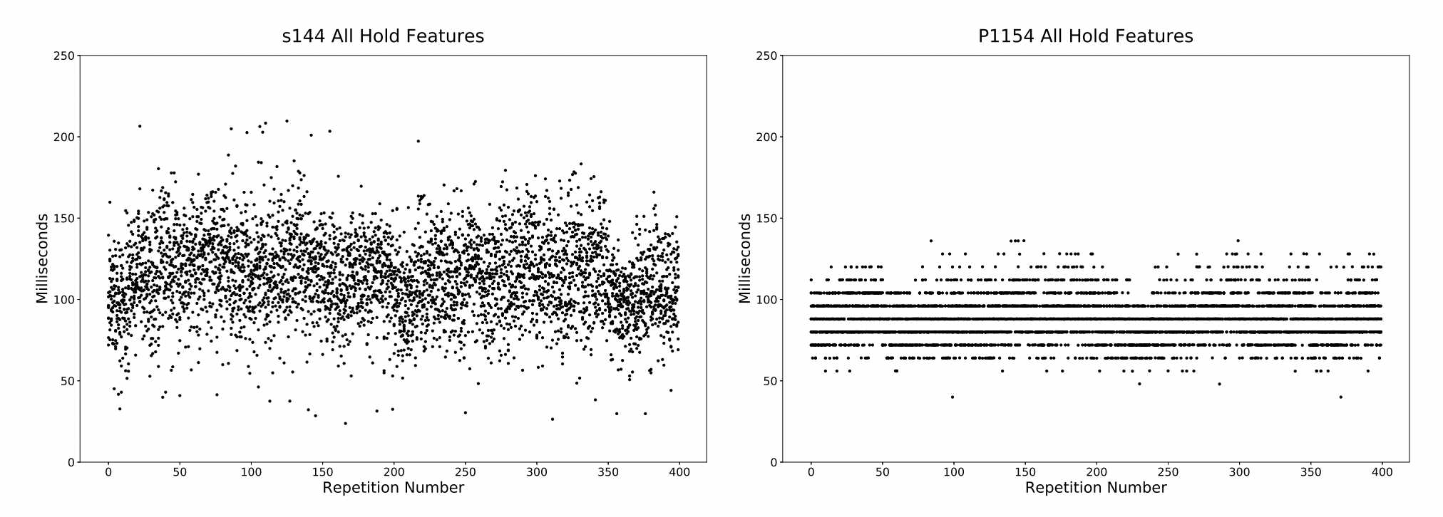
USB keyboards do not report keystrokes immediately upon a keypress. Rather, keystrokes are reported to the computer at a fixed timing interval set by the keyboard. This interval, called the polling interval, is most often a power of two. Since most subjects use USB keyboards, artifacts caused by USB polling are common in field data.

We examined the foremost datasets in the keystroke dynamics community and found that most contained USB polling artifacts, the only exceptions being our own 100-subject and 51-subject lab datasets for which an external timer was used to timestamp keystrokes. A list of datasets that were analyzed is presented below.

Keyboard Change:

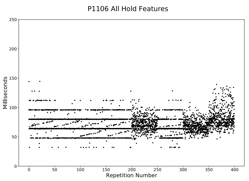
In the field, subjects may change keyboards during the experiment. Different keyboards have different properties: different keyboard matrix scan rates, actuation points, polling intervals, and baud rates to name a few. These differences can cause unpredictable changes in the collected data. In our dataset, these changes typically manifest in a mean shift of the data, change in observed polling interval, or both.

Bursts:

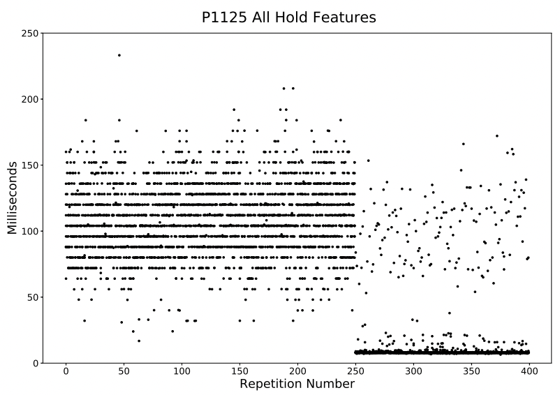
One of the hazards of collecting data in the field is that the processing load on a subject's computer cannot be controlled. In the cases that the processing load is high, input lag may cause many keystrokes to be recorded at once—in a burst. We see some occurrences of this in our field dataset, where many consecutive features are recorded in quick succession, all presenting times of around 0ms.

Ramps:

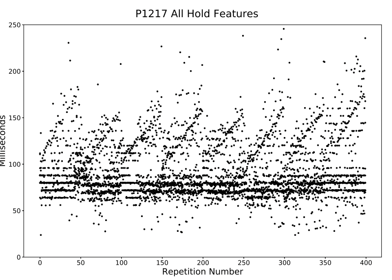
There exist several subjects for whom certain hold features have times that either regularly increase or decrease over the course of a session. The cause of this artifact remains unknown. Perhaps related to this anomaly is a widening gap around 0ms in the up-down latency times for those same subjects. Because the regular increasing/decreasing nature of the data when plotted is reminiscent of a ramp, we call these ramp artifacts.

Common questions:

• Q3-1: Can you tell me what the polling intervals for subjects in your field dataset are?
Yes. To accomplish this, we created two different programs to independently estimate polling intervals in our field dataset. Each program outputs both an estimate and a level of supporting evidence on a scale from 0-2. A 0 represents no evidence and a 2 represents the highest level of evidence. The output of both programs were combined to create a total level of evidence scale from 0-4, when the programs agreed on the polling interval. The following table presents the subjects whose polling interval was identified with the highest level of evidence—a score of 4—from both programs. Bear in mind that this not a comprehensive list of subjects and their polling rates, just those that we could identify polling intevals for with a high level of evidence.



Subject	Polling Interval Determined
P1102	8.0
P1103	8.0
P1104	8.0
P1107	10.0
P1108	8.0
P1110	8.0
P1111	8.0
P1112	8.0
P1113	8.0
P1114	8.0
P1117	8.0
P1118	8.0
P1123	8.0
P1127	2.0
P1130	8.0
P1131	8.0
P1132	4.0
P1133	8.0
P1134	4.0
P1135	8.0
P1137	8.0
P1144	8.0
P1147	8.0
P1148	8.0
P1150	8.0
P1152	8.0
P1153	8.0
P1154	8.0
P1156	16.0
P1157	8.0
P1158	8.0
P1159	8.0
P1160	8.0
P1162	8.0
P1178	8.0
P1180	4.0
P1181	16.0
P1182	8.0
P1183	4.0
P1188	8.0
P1189	8.0
P1190	8.0
P1191	8.0
P1192	8.0
P1193	16.0
P1195	8.0
P1199	8.0
P1202	8.0
P1204	8.0
P1206	8.0
P1209	16.0
P1210	8.0
P1211	8.0

• Q3-2: Could there be more artifacts, perhaps from other datasets, that are not presented here?
Certainly. This list is by no means comprehensive; it just presents the artifacts that we have observed so far. As more artifacts or explanations for current artifacts are brought to our attention, we may update this list.
• Q3-3: How can I avoid having these artifacts in my data?

There are a few steps that can be taken to diminish the effect of some of these artifacts, but many of the confounding factors that are at the source of these artifacts can never be fully eliminated. The only solution, then, is to use an external timer to timestamp keystrokes. If this is not an option, then the following measures may be taken:

• USB Polling: Have subjects use either PS/2 keyboards or USB keyboards with a low polling interval (such as gaming keyboards).
• Keyboard Change: Ensure that subjects do not change keyboards for the duration of the experiment.
• Bursts: Encourage subjects to close programs running on their computer before contributing data.
• Ramps: Since the cause of the ramps is unknown, we cannot provide any advice on how to avoid them. We encourage researchers to examine their data throughout their experiments to avoid collecting data with ramps.